Introduction
You can find the code for this project at: https://gitlab.com/ejt47/terrainshaderproject. I did try to clone, compile, and run the program when I started writing this, but it doesn’t seem to want to play ball. I promise it works on my machine though in the directory that it was built in!
This post provides detail on the process of development undertaken for the purpose of expanding an existing set of foundational techniques in shader programming, through the medium of practical application of advanced techniques within the context of a chunk of terrain. The work undertaken involved generation of a three-dimensional chunk of terrain from a two-dimensional grid using a height map texture through which normals were calculated and used in the application of colour, lighting, and fog; the use of tessellation shaders to provide a dynamic distant dependent level of detail and further generation of geometry; and the implementation of frame buffers with the intention to generate realistic shadows based on light position and geometry.
This was the final project for my Advanced Shader Programming Module in my final year at university.
Terrain
The Starting Grid
The starting point for the project was that of a two-dimensional grid extending outward in the x and z axes. The grid is constructed by a height, width and step-size which produces a flat plane made up of triangles dependent on the values fed to the constructor of the Terrain class for the aforementioned attributes. The width and height values fed into the constructor provide the iterative control values for an outer for loop controlling for z-axis depth and an inner nested for loop controlling for x-axis width with the step size being used additively to control for the application of offsets to the vertices that will make up the two triangles forming each quad that make up the cells of the grid. As the vertex positions are calculated per iteration of the loops they are pushed onto the back of a vector of float variables to be used in the generation of a Vertex Array Object (VAO) and a Vertex Buffer Object (VBO) to store the indices to be used in rendering the flat two-dimensional grid. This information is incredibly important as it is to be affected by further calculations to determine the height, normals, and overall potential complexity ceiling for the chunk to be rendered from the grid.
Height
It should be noted at this stage that the height variable mentioned previously in discussion of the attributes passed to the Terrain class constructor to form the base grid refers to one of two-dimensional axes giving the width and depth of the plane constructed by the perpendicular x and z axes.
The ‘height’ in the typical sense could be generated by either the application of procedural methods such as noise texturing and midpoint displacement or through the use of texture image maps such as height maps and displacement maps.
In the case of a map, a variation in bit-depth values is provided from each texel in a texture image that can be used to extend the grid upwards in the y-axis in order to render a two-dimensional image with the appearance of a three-dimensional chunk of terrain. In terms of height and displacement maps this is typically a distribution of greyscale bit-depth values that are used to set the y-axis value of a vertex position in terms of its numerical difference from white or black colour values.
Utilisation of maps for this use case holds certain positive aspects as some amount of care can be taken when designing a height or displacement map for a specific purpose giving it a bespoke quality with a relatively high level of finish. Once a map has been used once it can be used indefinitely if one alters the applied displacement scale value and colour that is to be applied, providing for a surprisingly significant level of variance between outcomes. This however, then ends up becoming a key drawback as a well designed height map will take a larger amount of time to create than the other option that is available, that of procedurally generating the displacement in the y-axis of the grid.
In terms of utilising procedural methods to displace the y-axis co-ordinate within a vertex position within the grid, there are two significant choices. One can either apply techniques utilising noise texturing or other effective methods such as midpoint displacement. Out of the two aforementioned procedural generation techniques, the most popular is likely the use of noise texturing techniques such as Perlin Noise or Open Simplex Noise, where the generation is driven by an algorithm that utilises the concept of octaves affecting amplitude and frequency of a pseudo-random gradient vector to produce the values by which to displace each vertex position in the y-axis.
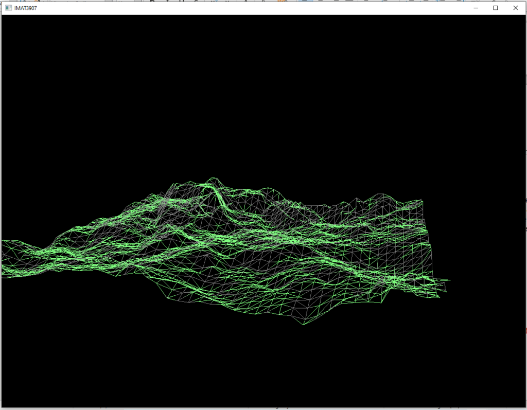
In this project it was decided that it would be more beneficial to make use of a height map texture than to implement a procedural generation technique in order to save time on development as a height map image had been provided by the course lecturer. It seemed that it would produce effective results at a faster pace in this regard and the outcome looked very much like terrain output. Included below are some images of the output as a wireframe when displacement in the y-axis is applied. When displacement had first been introduced lighting had not been implemented yet, and in this image it is possible to see the effect of the lighting model on the wireframe.
Fig 1.
Normals
A number of different methods have been applied over the course of the project’s development in terms of the calculations of normals in relation to the vertices of the triangles that can be seen in the above wireframe model. The final method that was settled upon was the Central Difference Method (CDM) within the Tesselation Evaluation Shader (TES) as this appeared to produce the most technically impressive, at least in terms of appearance, output. This is a method where the unit vectors in the up, down, left and right directions are calculated from the linearly interpolated texture coordinates associated with each vertex of the model, from the textureOffset function built in to glsl. An approximation of the cross product of the unit vectors, when scaled to fit the newly displaced y-axis values of the grid’s vertex positions, is given by the normalise function when it is passed a vec3 where the x-axis value is given by the right unit vector subtracted from the left unit vector, the y-axis is given by the value 2.0, and the z-axis value is given by the down unit vector subtracted from the up unit vector. This calculation gives an approximation of the point where all four unit vectors intersect which gives a result very close to the vertex normal of the triangle.
Fig 2.

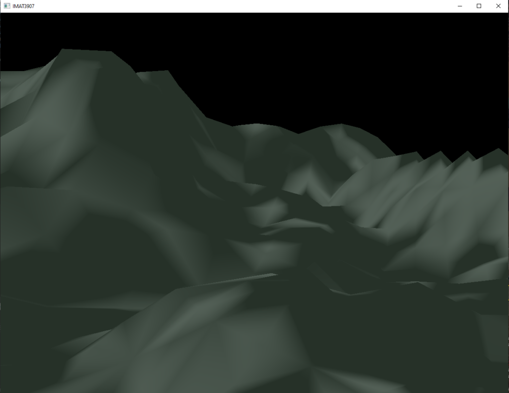
At various other stages in development the normals have been calculated in a variety of ways, including through geometry shaders, where surface normals have been calculated to output a flat colour shading effect. Figures three and four below demonstrate the difference between the two outputs at the same stage in development, where figure three demonstrates flat colour shading through vertex normals computed within the Geometry Shader and figure four demonstrates the output when vertex normals are computed within the Tessellation Evaluation Shader.
Fig 3.
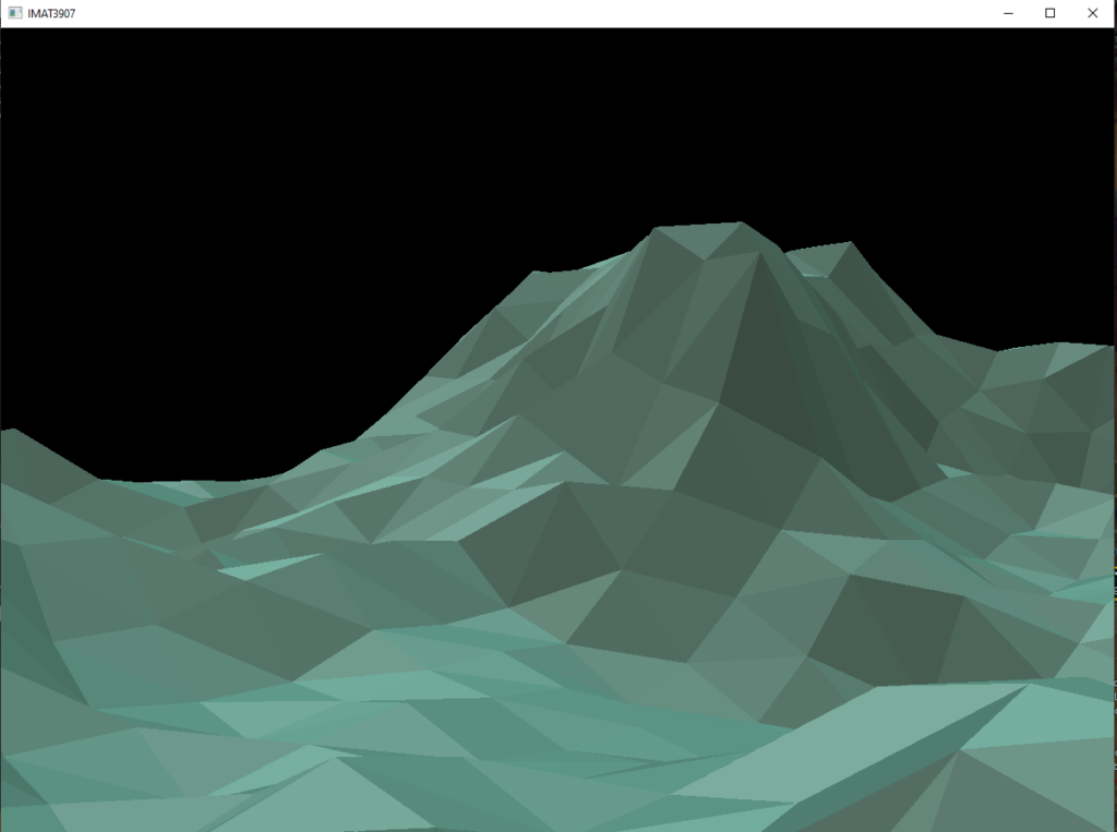
Fig 4.
Colour
As seen in figures three and four some level of colour has been applied to the model alongside some lighting which is to be discussed next.
The application of colour to the model happens within the Fragment shader and is dependent on multiple parts of the graphics pipeline, of course the final colour at each point on the model is dependent on lighting models and application of “fog” through distance dependent blending based on the clear colour of the graphics context. The below figures five and six are some examples of the different kinds of colours that a viewer might see if they were to navigate the camera around the scene.
Fig 5.
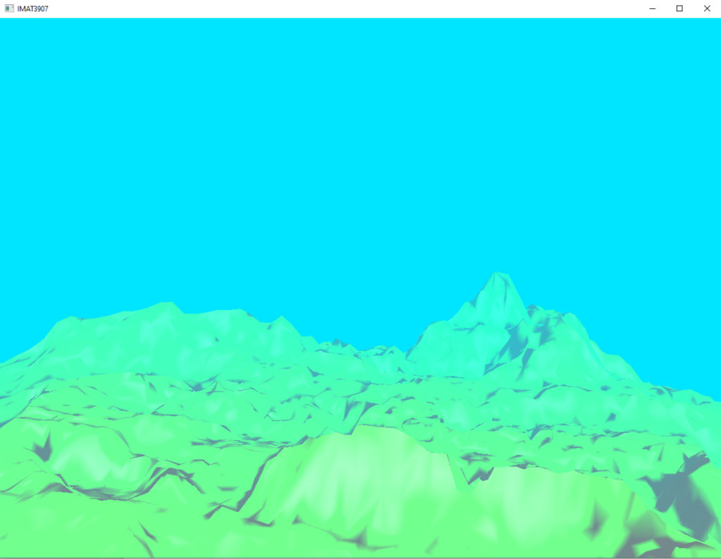
Fig 6.
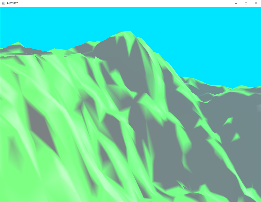
This part of the project on a personal note ended up being the part that frustrated me the most, and I lost quite a lot of hours to trying to get multiple colours rendering on a gradient slope dependent on the y-axis value of the vertex that was being read and affected by the Fragment Shader. At first this seemed as though it would not be all that difficult and in all honesty I still do not really know what went wrong, whether it was as a result of bad values being passed to my mix functions within the Fragment Shader or if it was that the way that the scale value is reduced back to its original range between zero and one for the purposes of calculation.
It is apparent to me that mixing by a gradient is possible as the green that is seen applied to the terrain is definitely the result of a mix between colours where smoothstep has been used, the gradient based on distance demonstrated as the terrain appears further away is also exemplary of this fact, however it was not possible within the time frame leading up to my deadline to correctly isolate the issue preventing the gradation of colour values dependent on the height of the terrain.
Lighting
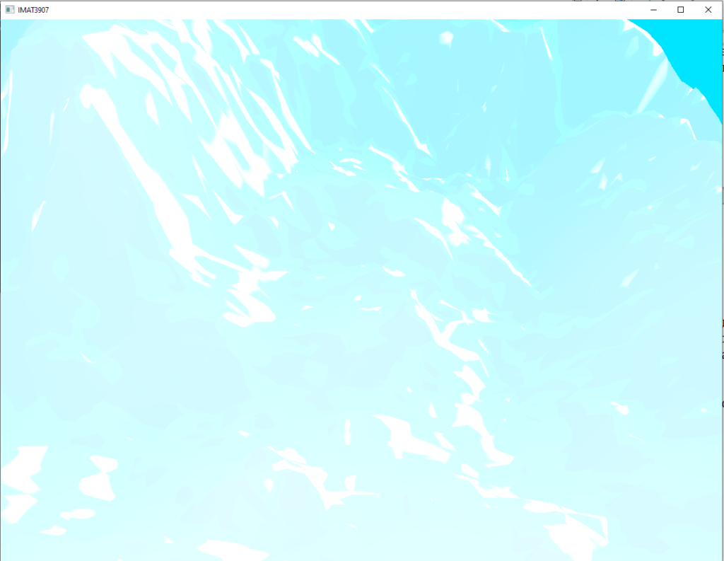
In terms of the lighting model that has been applied the choice was made to use a simple phong shading model that outputs the final fragment colour based on a combination of the lighting calculations for ambient, diffuse, and specular reflection off of the simulated surface. This is what produces the specular highlights seen and casting of shadows that is seen in figures five and six above. The diffuse lighting colour values have been set to the same values as that of the clear colour that is being used as a very basic “sky” within the scene, this made for a more appealing output than if the diffuse lighting colour had been set to be white, it was very important to tune the lighting values to appropriate colours for the final output, and tuning definitely made for easier blending within the fog implementation. Figure seven below gives an example of the appearance of the terrain when the lighting values are all set to white, which highlights the importance of finding the correct balance between lighting colour and the terrain’s material colour at each fragment.
Fig 7.
Fog
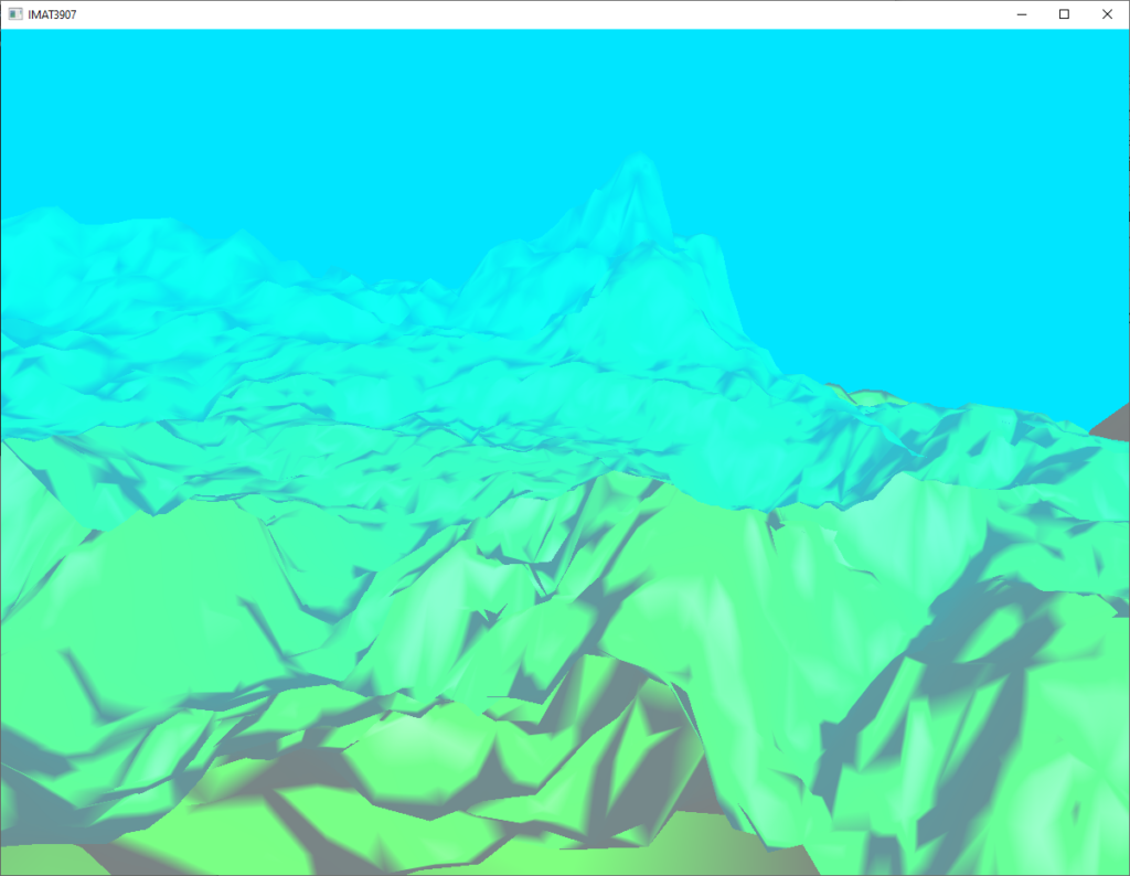
Implementation of fog has proved to be quite interesting. Given that the background colour of the scene is blue, if the distance at which the fog begins to blend at a higher rate is too close to the camera it can produce the effect of an underwater scene as displayed in figure eight below. Therefore it was actually relatively difficult to find the correct values to pass in to the exponential decay function to find the right balance, of which some progression is demonstrated by figures nine and ten. It was not at this point surprising to myself to see how little a change in these values would have drastic effects on the output scene due to tuning involved in my implementation of distance dependent level of detail in terms of generation of geometry within the Tessellation Control Shader which uses a similar approach in terms of determination of output based on distance from the camera view position. The fog itself is still not quite where I would like it to be, and it does seem to me that this could be further improved with a proper integration of depth frame-buffers for further control over post-processing effects.
Fig 8.
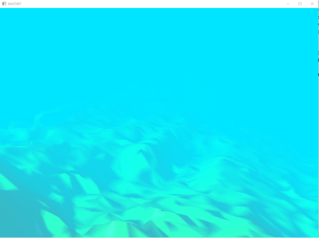
F ig 9.
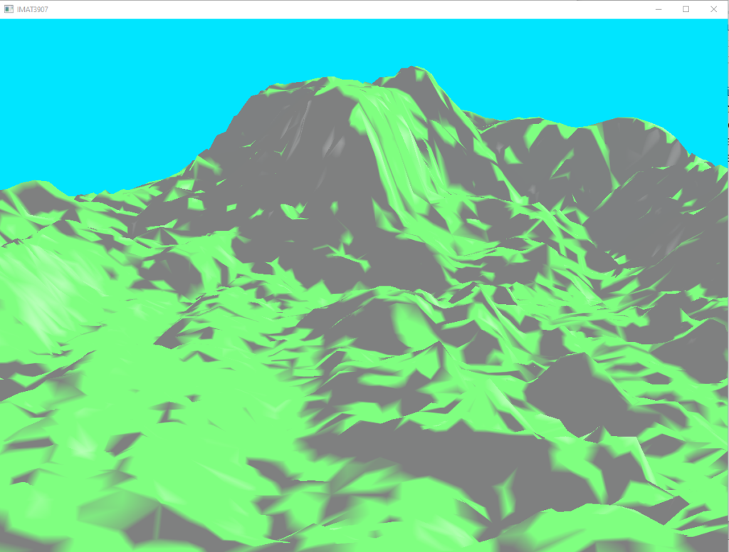
Fig 10.
Tessellation Shading
Tessellation Control Shader
The effect of the Tessellation Shaders have been really interesting to me throughout this project. Initially I struggled to find a suitable heuristic for the definition of an appropriate step in terms of incremental level of detail. Even currently it bothers me that I was unable to find a good way to smoothly transition between levels of tessellation detail through my experimentations.
Within the Tessellation Control Shader is where I have applied the exponential functions that increase the tessellation level based on distance. At this point I have managed to find some values to plug into my the exponential function that satisfies what I consider to be a suitable heuristic. I have first calculated an additive exponent to apply as the constant within the exponent function built in to glsl. This provide for some degree of staged stepping between levels of detail as demonstrated by the difference between figures eleven and twelve where the wireframe in figure eleven demonstrates three levels of tessellation at a suitable enough distance whilst the wireframe in figure twelve struggles to demonstrate two that were not a ridiculous distance away from each other.
Something that I really struggled in here with the way that I have calculated this additive exponent is that it seems quite counter-intuitive, seemingly doing the opposite of what I initially expected, in order to have the level of detail increase as the camera approaches the terrain I have had to further divide the calculated additive exponent by 5 thousand to find a heuristic that was aesthetically appealing to myself, whilst also making the additive exponent negative value alongside the calculated average distance from the camera, figure thirteen below gives a screen capture of the code snippet performing what I considered to be the best final exponential function. If I did not do these aforementioned things then the level of detail would end up decreasing as the camera approaches the terrain.
Fig 11.
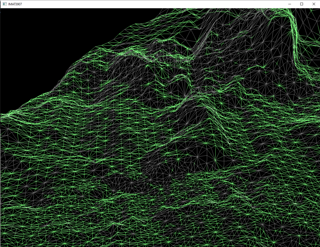
Fig 12.
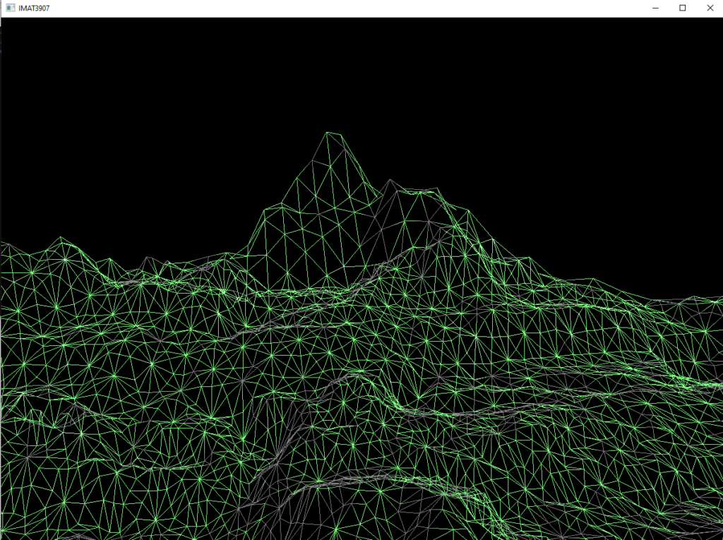
Fig 13.

Tessellation Evaluation Shader
The implemented Tessellation Evaluation Shader simply takes the output tessellation triangles from my Tessellation Control Shader and computes the interpolations between the the vertex positions and texture coordinates to then pass out geometry after computing the vertex normals to my fragment shaders by taking the patches from the primitive generator and applying the actual vertex data per patch for output.
Frame-Buffers
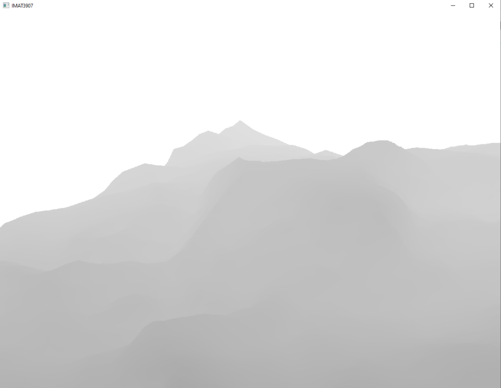
Although I was able to render my scene to a colour depth buffer and the final program is capable of creating a depth buffer object also as shown in figure fourteen, there is definitely something not quite right with the colour attachment buffer at the very least. When rendered to the colour frame buffer object the screen experiences tearing that previously had not been an issue, as demonstrated in figure fifteen. Unfortunately I did not have any extra time before the submission deadline to further explore this issue as it had been quite frustrating.
Fig 14.
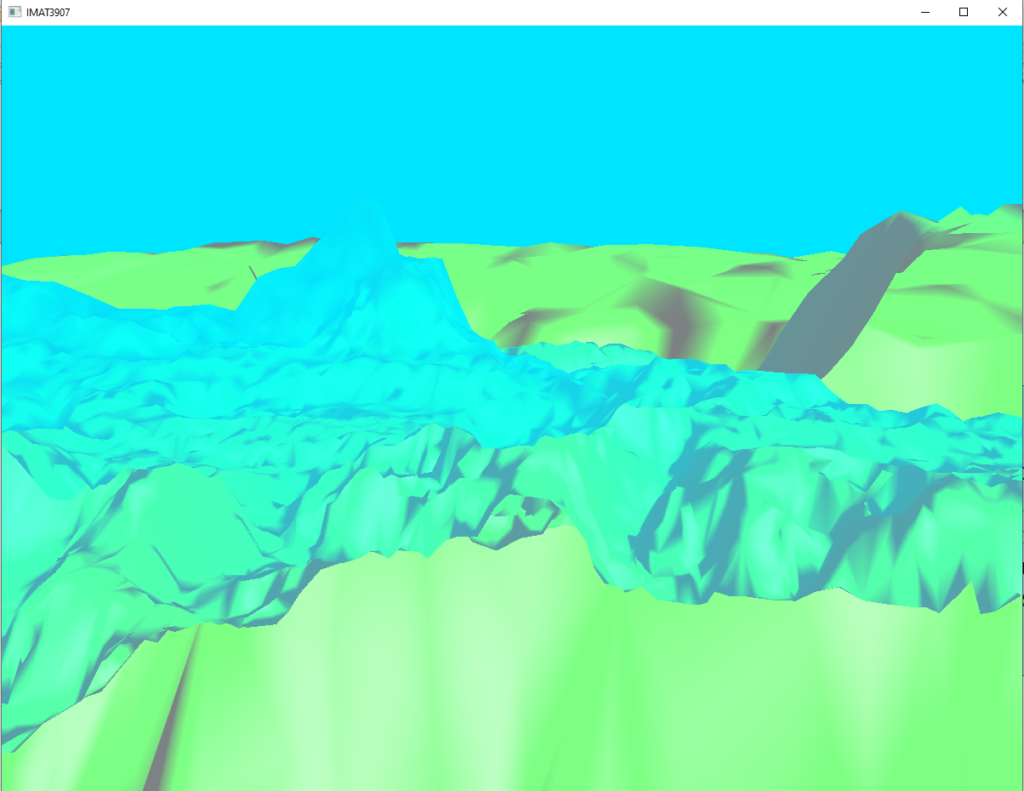
Fig 15.
Final Remarks
Whilst there are definitely issues with certain things in this project, overall I found the whole experience to be very informative and interesting. It was very interesting to see the progress as development continued. If I were to approach this project again from the start I believe that I would have taken more time to understand the mathematics behind the tessellation shaders and attempt to implement distance dependent detail for both lighting, fog, and level of detail through frame-buffers. Unfortunately I didn’t get to start working on frame-buffers until not long before the deadline and at the time when I felt that I properly understood what it is that they did and how they could be set up it seemed a shame that I didn’t spend more of my time tuning things within the context of these custom frame-buffers with application of more detailed post-processing effects in order to achieve the same goals with a more aesthetically pleasing outcome.