The nature of the coursework project had been to demonstrate the technical understanding and knowledge of mobile robotics that had been cultivated over the course of the module, in the form of a modelled pioneer robot within the CopelliaSim simulated environment. The completed work demonstrates a basic behavioural subsumption architecture through which obstacle avoidance, edge following, and mapping techniques have been implemented via the Lua scripting language.

The lecture content for the module presented a number of approaches to a behavioural subsumption architecture. The first possible architecture presented that could be applied would be a “hierarchical” loop where the robot’s sensors are used to detect changes in its surrounding environment, a plan is then developed according to the detection of the surrounding environment, and then the robot’s actuators put the developed plan into action, with the loop then returning to its beginning to then sense changes following actuation. The next possible architecture presented that could have been applied would be a “reactive” architecture where a back and forth occurs between sensors and actuators where the received sensor input data is interpreted as some form of sensed information that the actuators receive as input to then output actuation commands. Lastly the final presented option would be a “hybrid” approach that combines elements of the two aforementioned approaches to the subsumption architecture, specifically this can be described as a feedback loop wherein a plan exists for possible scenarios in terms of sensory input, the plan then can be referred to in order to output some forms of directives according to the back and forth between the sensor and actuation elements of the architecture which operates actuation commands according to the system directives for the scenario that is most relevant for the interpreted sensory input.
The implementation for this piece of coursework made use of the hybridised approach, where there is a specific directive for specific scenarios. These directives are decided upon based on the sensory input which feeds into a number of layers within the subsumption architecture in order to flip boolean variables that are indicative of finite states of action for each possible directive. This very basic finite state machine is then able to perform tasks relating specifically to edge following, obstacle avoidance, and mapping, to be further outlined below.
The simulated robot’s avoidance strategy is driven by Proportional, Integral, Derivative (PID) feedback control. The goal of a PID feedback loop is to control the power applied to each wheel of the robot with a certain level of stability so that the robot will travel in as straight a line as is possible when following an edge, and turn to avoid obstacles by reducing power to zero in the wheel motor so as to turn around the correct axis to best avoid obstacles according to the sensory input of the robot. This is a bit similar to how one might make a turn while rowing a boat, except, you’re a robot and you are trying to avoid crashing into stuff.
Where the robot’s goal is to maintain an appropriate distance from a set point in terms of distance, the PID feedback control makes use of the calculus principles of integration and derivation in order to control the error over time so as to assure the correct proportion of power is applied in the correct operational directives.
The main avoidance occurs when the robot’s sensors detect an obstacle directly in front of it where it then turns to follow the edge essentially by the same principle of the sonar sensor detection, but instead of the sensors on the front of the robot controlling the avoidance, a distance is maintained by the PID feedback controller according to the given distance to maintain from said edge.
The proportional element of the controller refers to the output in terms of power to the wheel motors, the integral element of the control refers to the reduction of error over time within the feedback control loop, and lastly the derivative element of the controller refers to change in error over time.
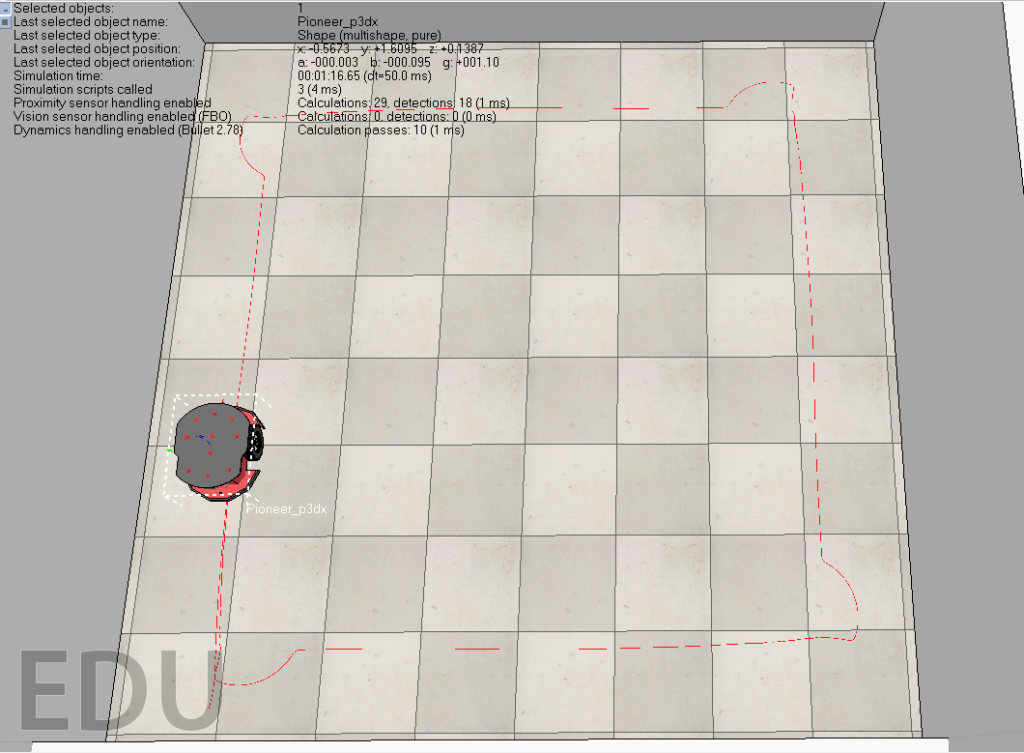
An important aspect of this application of PID feedback control was to tune the individual aspects that make up the PID controller, the proportional, integral, and derivative elements. These controls are provided in the form of gain values. Gain can be thought of as a measure of amplification of signal strength, which in this context these measures when combined and tuned correctly will amplify the proportional power to the wheel motors according to the directive requirements for each scenario the robot may encounter whilst controlling the error over time which will be seen in terms of oscillation. The figures below demonstrate the difference between the robot’s path before(fig. 1) and after(fig. 2) tuning the PID feedback controller. Although it may be difficult to see with relatively small images, the first image shows a high amount of smaller oscillations, whereas the second image demonstrates essentially no oscillation and smooth straight pathing.
Fig. 1 Before Tuning.
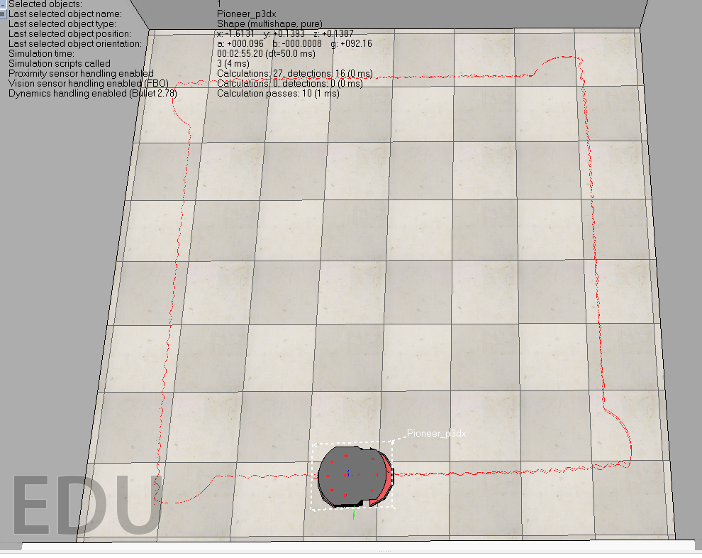
Fig. 2 After Tuning
The strategy applied for the tuning of the PID controller was the method recommended in the module lecture on PID, where the proportional gain value is first set to a low value, the derivative gain value is then set to one hundred times the value of the proportional gain, the derivative gain value is the raised until the system demonstrates a fast and large oscillation, after which the derivative gain value is reduced by either a factor of two or four. If the system continues to oscillated the proportional gain value is then reduced by a factor of ten until the oscillation stops, if the system is then stable the proportional gain value is increased by a factor of ten until oscillation begins again, and then dropped by a factor of two or four until stable again. Once a suitable level of stability has been ascertained, the integral gain value is the set to a very low number, around hundredths or thousandths of one, this is then increased by a factor of ten until oscillation begins again, where it is then dropped and further fine tuning of the values occurs until the system seems to be stable. The final values for proportional, integral, and derivative gain that were most suitable for my system ended up being; 5, 0.015, and 2.5 respectively.
Once the edge following and avoidance strategies had been implemented a basic scatter-gram mapping was introduced to the implementation. This requires the calculations of the simulated robot’s position and orientation, the sonar readings giving distance from any obstacles, and the sonar angles for each sensor attached to the pioneer robot simulation.
The sonar angles can be calculated quite easily and stored in an array, given that there are sixteen sensors on the robot, this then means that sixteen sonar angle values must be stored within an array in order to use this information for mapping. Two different value range were used to find the most appropriate values for this element of the mapping implementation, one set of values ranging from three hundred and sixty down to zero; and another ranging from positive to negative one hundred and eighty, the below figures demonstrate the difference in real-time output between the two.
Fig 3. +/-180
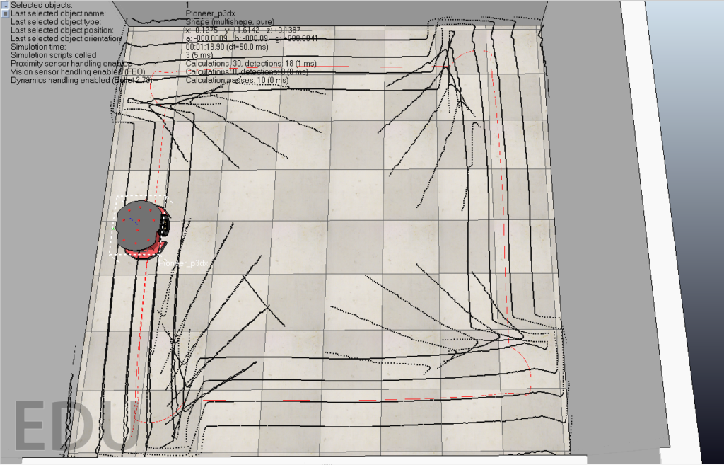
Fig 4. 360 to 0
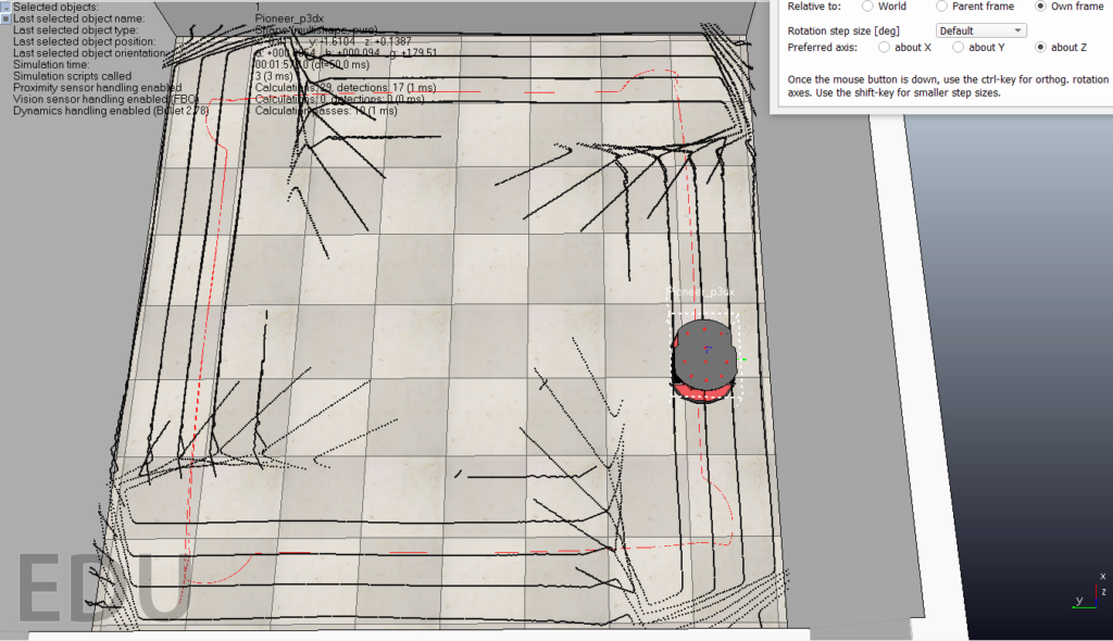
The difference here isn’t particularly noticeable at first glance, however it was apparent to me that using the full range of three hundred and sixty degrees as positive values as opposed to a full range of three hundred and sixty gives a more developed view of the sonar hits on both sides of the robot.
The above mapping points are calculated by obtaining the sonar hit in the x and y axes using trigonometry, after which the rotation matrix is applied in the gamma plane, as in the two-dimensional space created by the intersection of the perpendicular x and y axes, to the first calculated sonar hit positions in x and y, before finally being added to simulated robot’s position within the space. After these calculations are made the points can then simply be drawn to the screen, and further provision is made to output these points to a csv file which can be used to plot a scatter graph that gives a view of the path the robot takes over the course of the simulation, demonstrated by the figure below.
Fig 5. Example of an output scatter plot
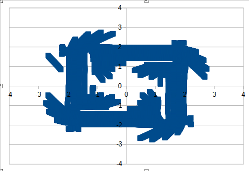
Unfortunately I was unable to implement anything beyond this due to time constraints, I had hoped to implement wandering, but ended up spending too much time working on getting the mapping functionality to a point where I was confident that what I was seeing was worthwhile. Alongside this I spent a bit too long trying to ensure that the robot, when following the edge on its right hand side, would turn to the left and travel anti clockwise around the space, at points this was possible however it came at a sacrifice of avoidance if the robot’s position was translated to a point within the space where it would not follow an edge and it would just drive straight into the wall and never attempt to turn, likely due to the fact that my solution to get the robot to turn both left and right depending on the edge it was following involved sensors that were too close to eachother, thus when a slight adjustment in orientation was made, upon the next frame the robot would then attempt to turn the other way due to it believing that the closest edge was now the edge opposite to the previous frame’s closest edge. I would have liked to perfect this but deemed it necessary to move onto mapping at risk of ending up with an entirely unfinsihed project.
In conclusion, there are many different techniques that can be applied to a simulation such as this, and it definitely would be interesting to continue attempts to implement these things that I have mentioned ended up being left unfinished. I would have liked to attempt to implement proper wandering and more consistent and performative edge following across different scenarios. A better mapping implementation could have really made the robot’s performance sky-rocket, if for example an occupancy grid had been used.
Post-graduation I have not had as much time on my hands as I would have liked to pursue projects, and I think that robotics isn’t where I would like to place my focus. However, I had loads of fun, and reading back through my notes and code for this project helped massively to organise some of the logic and piece back together how some of these things I built work.
I’ve included the Lua script that defines all of the behaviour outlined above. I had to change a local filepath to some placeholder spam. I also apologise in advance for how descriptive & scatter-brained my comments are here, I have a bad habit of making my notes in my source code.
function sysCall_init() -- sysCall_init is called once when start button is pressed, initialising the system by initialising the required starting functionality of the robot
    usensors = {-1,-1,-1,-1,-1,-1,-1,-1,-1,-1,-1,-1,-1,-1,-1,-1} -- fill the array usensors with a default value -1(indicative of reserved memory but unassigned)
    for i = 1,16,1 do -- for loop iterates 16 time starting at 1, steps of size 1
        usensors[i]=sim.getObjectHandle("Pioneer_p3dx_ultrasonicSensor"..i) -- assigns the object handle for a pioneer robot's ultrasonic sensor at each index position of usensors
    end -- end for loop
    motorLeft = sim.getObjectHandle("Pioneer_p3dx_leftMotor") -- motorLeft variable instantiated and initialised to the left wheel motor of the pioneer robot
    motorRight = sim.getObjectHandle("Pioneer_p3dx_rightMotor") -- motorRight variable instantiated and initialised to the right wheel motor of the pioneer robot

    v0 = 2 --v0 variable instantiated and initialised to the value 2, gives a velocity value
    setPoint = 0.5 -- setPoint variable instantiated and intialised to 0.5, giving the distance value that is wished to be maintained as the offset from the wall
    sonarReadings = {-1,-1,-1,-1,-1,-1,-1,-1,-1,-1,-1,-1,-1,-1,-1,-1} --instantiate and initialise with default -1 values an array to store sonar readings

    --gain values, can be changed, to find a sweet spot!
    --gain gives a control variable by which oscillation can be reduced
    p_gain = 5 --proportonal gain
    i_gain = 0.015 --integral gain
    d_gain = 2.5 --derivative gain

    previousError = 0 -- variable to record the previous error

    pastErrors = {0,0,0,0,0} --array to store a sequential series of previous errors for the integral component of the controller
    integralCount = 1 --Iteration counter for counting through the pastErrors array in order to compute the integral component of the controller

    follow = false
    wander = false
    avoid = false

    --you will need to extend this to the full 16 sonar angles DO NOT 4GET 3HEAD
    sonarAngles = {360, 337.5, 315, 292.5, 270, 247.5, 225, 202.5, 180, 157.5, 135, 112.5, 90, 67.5, 45, 22.5}
    --180, 157.5, 135, 112.5, 90, 67.5, 45, 22.5, 0, -22.5, -45, -67.5, -90, -112.5, -135, -157.5, -180
    --{360, 337.5, 315, 292.5, 270, 247.5, 225, 202.5, 180, 157.5, 135, 112.5, 90, 67.5, 45, 22.5

    --initialise filepath var with path string (cannot do ..\\mapOut.csv for some reason, so therefore a direct relative path)
    filepath = "blahfilepath\\blah.csv"
    file = io.open(filepath, "a+") --a+ gives command to append / gen new file if not exisiting already
    io.output(file)

    drawing = sim.addDrawingObject(sim.drawing_points, 2, 0.0, -1, 100000)

end


function sysCall_cleanup()
 io.close(file) --needs to be made sure the file is closed correctly
end

function sysCall_sensing()

    readSensorData()
end


function sysCall_actuation() --sysCall_actuation function then defines the behaviour of the robot, in terms of how the attributes as defined in sysCall_init are affected
    --followEdge()
    setBehaviourFlags()

   -- Initialise the velocity values on each wheel to the constant 2
    vLeft = v0
    vRight = v0

    if(avoid) then
        avoidObstacle()
        print("Avoiding collision")
    end

    if(follow) then
        followEdge()
        print("Following edge")
    end

    if(wander) then
        --wanderArea()
        print("Wander func not yet implemented")
    end

    sim.setJointTargetVelocity(motorLeft,vLeft) -- set the target velocity of the motor actuating the left wheel to the now calculated vLeft velocity value
    sim.setJointTargetVelocity(motorRight,vRight) -- set the target velocity of the motor actuating the right wheel to the now calculated vRight velocity value
end

function readSensorData()

    for i=1,16,1 do -- for 16 iterations
        res,dist=sim.readProximitySensor(usensors[i]) -- instantiate and initialise the res(result) and dist(distance) variables to the return of the reading from
                                                      -- the proximity sensors in the usensor array at index i
        --store sonar values
        if (res > 0) then -- perform check that res > 0 (otherwise leaves system open to crash)
            sonarReadings[i] = dist -- store the dist value to the ith index of sonarReadings
            mapSensorData(i)
        else
            sonarReadings[i] = 0 -- otherwise set the value at the ith index of sonarReadings to 0, so that nothing is then done
        end
    end

end

function setBehaviourFlags()
     --check front sonar (sonar 4(left) and 5(right)) to see if anything is in front of the robot
    if (sonarReadings[3] > 0 and sonarReadings[3] < setPoint) then -- if readings at index 3(left-left-side front-facing) is more than 0, and less than the setPoint(error(wall2robot offset)) value
        follow = false
        avoid = true
        wander = false
    elseif (sonarReadings[4] > 0 and sonarReadings[4] < setPoint) then -- if readings at index 4(left-side front-facing) is more than 0, and less than the setPoint(error(wall2robot offset)) value
        follow = false
        avoid = true
        wander = false
    elseif(sonarReadings[5] > 0 and sonarReadings[5] < setPoint) then -- if readings at index 5(right-side front-facing) more than 0, and less than the setPoint(error(wall2robot offset)) value
        follow = false
        avoidRight = true
        wander = false
    else
        follow = true
        avoid = false
        wander = false
end

function followEdge()
    -- if left wall is > 0 (closer) and distance < right wall then wall following to the left
    if (sonarReadings[1] > 0 and sonarReadings[1] < setPoint) then
            print("left wall closer, distance to wall: ", sonarReadings[1])
            error = setPoint - sonarReadings[1]
            --proportional control is == to error(wall2robit offset) * p_gain
            p = error * p_gain

            --integral control
            --integral(sum of errors and threshold(avg))
            integralSum = 0
            if(integralCount > 5) then
                integralCount = 1 --reset to 1 if counter has exceeded size of the pastErrors array
                pastErrors[integralCount] = error -- write to the array of pastErrors the error just calculated
            else
                integralCount = integralCount + 1 --increment counter because array has not yet been fully iterated through
                pastErrors[integralCount] = error -- write to the array of pastErrors the error just calculated
            end
            --iterate through array of pastErrors
            for i = 1,5,1 do
                integralSum = integralSum + pastErrors[i] --obtain the total sum of past errors by iteration and incrementation by addition assignment
            end
            integralAvg = integralSum / 5 --find the threshold average of the past errors --is there a way to do this by size of array?
            i = integralAvg * i_gain --integral control = integralAvg * i_gain

            --derivative control is == to previous error - current error
            d = (previousError - error) * d_gain

            --calculate final velocity
            vLeft = v0 * (p + i + d)

            --Update previousError
            previousError = error
        --end
    --else right wall must be closer then wall following to the right
    elseif (sonarReadings[8] > 0 and sonarReadings[8] < setPoint) then
            print("right wall closer, distance to wall: ", sonarReadings[8])
            --calculate proportional control
            error = setPoint - sonarReadings[8]
            p = error * p_gain

            --integral control
            --integral(sum of errors and threshold(avg))
            integralSum = 0
            if(integralCount > 5) then
                integralCount = 1 --reset to 1 if counter has exceeded size of the pastErrors array
                pastErrors[integralCount] = error -- write to the array of pastErrors the error just calculated
            else
                integralCount = integralCount + 1 --increment counter because array has not yet been fully iterated through
                pastErrors[integralCount] = error -- write to the array of pastErrors the error just calculated
            end
            --iterate through array of pastErrors
            for i = 1,5,1 do
                integralSum = integralSum + pastErrors[i] --obtain the total sum of past errors by iteration and incrementation by addition assignment
            end

            integralAvg = integralSum / 5 --find the threshold average of the past errors --is there a way to do this by size of array?
            i = integralAvg * i_gain --integral control = integralAvg * i_gain

            --calculate derivative control
            d = (previousError - error) * d_gain

            --calculate final velocity
            vRight = v0 * (p + i + d)

            --Update previousError
            previousError = error
        end
    end

end

function avoidObstacle()

    if(avoid) then
        vRight = 0 -- turn to the right, by stopping the right motor(set velocity to 0)
        vLeft = v0 -- left wheel then continues moving (opposite forces, think rowing a boat)
    end

end

function mapSensorData(iter)
    if(iter < 17) then

        --calculate the positions in the x and y for the sonar rays used for sensing, 0.15 gives robit radius
        sonarX = math.cos(math.rad(sonarAngles[iter])) * (sonarReadings[iter] + 0.15)
        sonarY = math.sin(math.rad(sonarAngles[iter])) * (sonarReadings[iter] + 0.15)

        --get the xy plane rotation of the pioneer robit
        rotation = sim.getObjectOrientation(sim.getObjectHandle("Pioneer_p3dx"), -1)
        g = rotation[3]
        rotX = sonarX * math.cos(g) + sonarY * -(math.sin(g))
        rotY = sonarX * math.sin(g) + sonarY * math.cos(g)

        --get the robit's translation and add to the calculated xy plane rotations to get final x and y positions
        position = sim.getObjectPosition(sim.getObjectHandle("Pioneer_p3dx"), -1)
        finalX = rotX + position[1]
        finalY = rotY + position[2]

        --write to file
        io.write(finalX, ",", finalY, '\n')
        --draw to screen
        sim.addDrawingObjectItem(drawing, {finalX, finalY, position[3]})
    end
end